(pressing HOME will start a new search)
![]()
![]()
- ASC Proceedings of the 23rd Annual Conference
- Purdue University - West Lafayette, Indiana
- April 1987 pp 131-139
|
(pressing HOME will start a new search)
|
|
A
MODEL FOR RETIRING, REPLACING, OR REASSIGNING CONSTRUCTION EQUIPMENT: A NEW LOOK
AT AN OLD PROBLEM
|
Michael
C. Vorster and
Glenn A. Sears University
of New Mexico |
|
Reprinted
from Journal of Construction Engineering and Management, |
Introduction
Models
aimed at quantifying the various decisions which must be made by managers of
construction equipment have appeared in the literature for over 60 years. It may
be presumed that inflation and trying economic times have sharpened skills, but
alas this is not so. The basic definition of economic life and the rationale
behind it have remained unchanged since Taylor's 1923 paper in which he stated:
All
we have to do on this basis is to compute X (the average annual cost) at the end
of each year for the total time the machine has been used up to that date and
discard the machine when X ceases to decrease and begins to increase, provided
labor costs and the like have remained constant. If these costs have increased,
however, we can well continue to use the old machine after the minimum has been
passed. It is then only necessary to compute the unit cost for each year from
that point on and discard the machine when the annual unit cost becomes greater
than the estimated unit cost for a new machine under the changed economic
conditions.(1)
We
may be tempted to say that nothing has changed. Extensive work by authors such
as Terborgh(2) and Douglas(3) have added to the literature and done much to
increase the rigor of the analysis but in essence it is true, nothing has
changed.
From
a practical point of view there has also been little change. Extensive
interaction between the authors and practitioners in the field lead them to
believe that the conclusion drawn by Preinreich in 1940 is as valid now as it
was then. He stated:
�On
the whole then I am not greatly impressed by the practical merits of the theory
of economic life, although it is no doubt a fascinating subject worthy of study
for the sake of its legitimate place in economics. From any other viewpoint, it
seems to share the well known peculiarity of the weather: A great deal may be
said, but very little can be done about it!(4)�
Existing
methodologies fail because they ignore too many important practical factors in
order to satisfy a perceived need for quantitative precision. New thinking must
be introduced to include the many factors which influence equipment decisions
but which do not appear as hard data in any cost accounting system.
The
model proposed in this paper seeks to do this by presenting a formal mechanism
for including the effect of deteriorating mechanical performance in order to
determine the effective cost of a particular machine working in a particular
application. This makes it possible to review the manner in which machines are
assigned to applications and to identify those machines which are candidates for
retirement or replacement on the grounds that they are no longer cost effective
in any available application.
Equipment Management Objectives
One
of the main reasons why existing models are not widely used in practice stems
from the fact that the objective function used seldom reflects many of the real
issues which must be addressed when managing construction equipment in a working
environment. Classic minimum equivalent annual cost models, for example, presume
that the owning and operating cost of a particular machine is the only important
variable and that it is this which must drive all decisions.
Profit
maximization models, such as that developed by Douglas(3), improve the situation
slightly by proposing profit as the objective function. They fall short of
reality by largely neglecting the fact that construction equipment works in
closely knit teams with the sole objective of completing construction on time
and on budget.
It
has been proposed(5) that equipment has but one fundamental reason for being: to
facilitate the construction process and that all equipment decisions must be
taken with this in mind. Objectives for the management of construction equipment
should be set so as to maximize construction profits rather than minimize
equipment costs. Models to assist en decision making should reflect this and
should focus on both the machine and the productive team within which et works.
Consequential costs
Equipment
costs are normally divided into two categories, owning and operating. The former
covers transactions such as purchase, finance and resale while the latter covers
costs such as fuel, consumables, repair and maintenance. A third category,
consequential costs, may be defined to cover the intangible costs arising from
the fact that equipment often performs less well than expected and thereby
impacts on many aspects of the production process.
The
existence of consequential costs is widely acknowledged but often disregarded.
They tend to introduce an untidy, imprecise component to any analysis and as
they do not appear as hard data en the cost accounting system, invariably play a
minor role in formal decision making. Their role in informal decision making and
en influencing perceptions about equipment cannot, however, be underestimated.
They must thus form part of any model which seeks to reflect reality even if
they do introduce assumptions and inaccuracies of concern to those striving for
quantitative precision. It is simply not possible to develop a perfect model of
an imperfect world.
Many
authors mention consequential costs. The basic premise is that equipment failure
forces construction supervisors to change previously laid and presumably optimum
construction plans and that et is these changes which give rise to consequential
costs. Early treatments of the consequential cost phenomena use terms such as
"payroll during delays caused by breakdown"(6) while others define a
component called "downtime cost" as part of operating cost(7).
Nunnally states that:
�One
method of assigning downtime cost to a particular year of equipment life is to
use the product of the estimated percentage of downtime multiplied by the
planned hours of operation for the year multiplied by the hourly cost of a
replacement or rental machine(8).�
This
approach focuses on the failed machine itself and does not recognize the impact
that the failure may have on other members of the working team. It thus tends to
underestimate the costs involved.
Cox
calculates the cost of "interruption caused by component failure" as
being the product of the annual frequency of component failure, the average time
to replace the component and the total cost of the team affected by the
failure(9). This may be construed as being a little harsh as the total cost of
the team affected cannot be put against the failed machine for the full repair
period, since skilled field supervisors well take action and replan the
productive teams given the changes brought about by the equipment failure.
The
methodology which forms the bases of the model described here is similar to that
proposed by Cox. The total cost of the team affected by the failure is, however,
adjusted by means of a carefully defined failure cost profile for a given type
of machine en a given field construction application.
The Failure Cost
Profile
|
|
|
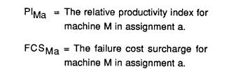
FIG. 1: Failure Cost Profile |
The
Failure Cost Profile (FCP) is a diagram designed to show how the total cost of
all the resources affected by the failure of one member of a productive team
varies with the duration of the failure. An example is given in Figure 1 using
costs aggregated on an hourly basis.
From
Figure 1, it can be seen that
|
It
can be seen that equation (1) differs from the methodology proposed by Nunnally
in that Fc includes all the affected resources (not only the failed machine) and
FCP varies with Hr. Equation (1) also varies from the methodology proposed by
Cox(9) in that FCP is able to vary with time as the impact builds up or as
action is taken to re-plan the productive teams.
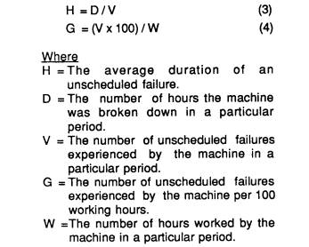
Drawing Failure Cost
Profiles
It
is certainly no simple matter to determine failure cost profiles for a large
number of machine types in numerous applications. Limited field work was done to
determine the acceptance of the concept and to assess whether or not reasonably
accurate estimates could be made. The results
were
most encouraging and a few profiles are given as examples in Appendix 1.
The
profiles were obtained by meeting with production and equipment managers and
seeking consensus to four simple questions.
|
Time
was frequently needed to reach consensus on questions one and two. Once this had
been done, answers to question three indicated good confidence with very strong
support for question four.
As
expected, failure cost profiles differed dramatically depending on whether a
machine was assigned as
|
|
|
Defining
the profiles served to illustrate the relative importance of failure frequency
and failure duration in the mechanical performance of a machine. This issue has
been the subject of substantial debate which, using the failure cost profiles,
may be summarized as follows
|
These
then are the, basic concepts for the development of a reassignment model for
construction equipment.
The Reassignment
Model
As
indicated earlier, the model has been designed to assist in decision making
regarding the manner in which particular machines are assigned to field
applications. In the general case the model can be used to identify machines
which are candidates for retirement or replacement when they are no longer cost
effective in any available application for a particular contractor. This is
achieved by combining the tangible costs of continued ownership and operation
with the consequential costs arising from age and deteriorating mechanical
performance. This is done in the following form
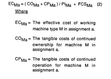
|
|
The
calculation of COMa and CPMa will not be discussed here as
many well known methodologies exist(10). Suffice to say that the focus should
fall on the cost of continued ownership and operation in cases where the minimum
equivalent annual cost point has been exceeded.
PI
Ma is introduced in order to compensate for the fact that the
productivity of machines of essentially similar type but different age varies
from application to application due to technological development. The index is
presented in the form of a relative productivity matrix obtained by assessing
the productivity of each machine in each application. The matrix should not
include an allowance for mechanical quality since this is taken into account as
a separate factor in the failure cost surcharge (FCSMa). It must be
stressed that the matrix is intended to allow for relatively small variations in
productivity between essentially similar machines; it cannot be used to make
adjustments between machines of a different class or inherent capability.
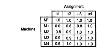
An
example of a relative productivity matrix is given in Table 1 from which it can
be seen that:
|
|
|
|
|
|
|
Determination
of the the failure cost surcharge ( FCSMa) necessitates the use of
the failure cost profile discussed previously together with two very simple
measures for the mechanical performance of a particular machine. If it is once
again assumed that costs are aggregated on an hourly basis, these may be
expressed as:
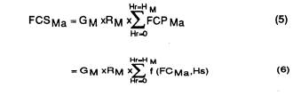
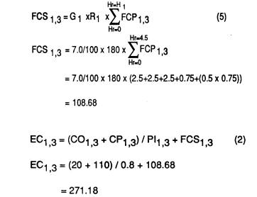
Given
the above, the failure cost surcharge in $ per 100 working hours can be
calculated from the area under the failure cost profile as follows:
use
as a replacement for an existing machine of the same type. This machine,
normally called the challenger, will be identified as M* if it is of type M as
opposed to existing machines of type M which are identified as M1, M2, M3, Once
this has been done it is necessary to calculate the effective working cost of
the challenger for all assignments
|
|
It
should be possible to see that
|
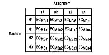
The next step is to calculate the effective working cost of all existing machines of the given type (defenders) in all suitable assignments The results are placed in a matrix together with the values obtained for the challenger as shown in Table 2.
It
should be possible to see that defenders, and particularly old defenders will
have
|
|
TABLE 2.-Effective Cost of Working Machine M in Assignment a |
|
|
|
Using the
Reassignment Model
The
first step necessary for the use of the model is to identify a new machine
suitable for
|
|
The
figures appearing in the matrix can be reviewed in order to obtain information
regarding:
|
Conclusion
It
was argued that existing models used for decision making in equipment management
do
not
adequately reflect reality and that this is the reason why they have not found
application in practice. It seems intuitively sound that machines should be
assigned to different tasks in a structured way which takes account of:
|
The
reassignment model takes these factors into account and seeks to quantify the
consequential costs of machine failure by means of a carefully defined failure
cost profile. It is accepted that the profile introduces an element of judgment
into the model and that this reduces its accuracy in purely quantitative terms.
It is however felt that the existence of consequential costs cannot be neglected
entirely and that the methodology used in the model has advantages over
previously published work.
The
worked example given as Appendix I shows the use of the model with regard to
both replacement and reassignment.
Appendix 1: Example
Application
of Reassignment Model to Front End Loaders used at Beta Quarries
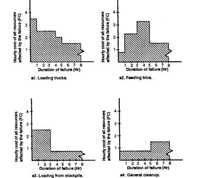
Beta Quarries operates four two cubic yard front end loaders on various assignments which are classified as follows
|
Discussions have been held regarding the implications of mechanical failure in a loader performing any one of the above tasks. Arising from this it has been agreed that the failure cost profiles shown in Figure Al are reasonable and can be used in the reassignment model.
Quarry
management is considering the purchase of a new loader to replace one or more of
the existing machines which vary in age from M1, the oldest to M4 the youngest.
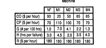
The data shown in Tables Al and A2 have been extracted for the existing loaders
and for a desirable challenger. The following assumptions were made:
|
The
above information, as well as the failure cost profiles given in FIGURE Al, have
been used to calculate the effective working cost for a given machine in a given
assignment using equations (5) and (2).
|
|
|
FIG.
Al. Failure cost profiles for 2cy. front end loaders at Beta Quarries. |
|
TABLE
A1.-Basic Data |
|
|
|
TABLE A2.-Productivity matrix |
|
|
e.g.
The effective working cost for machine 1 in application 3
|
|
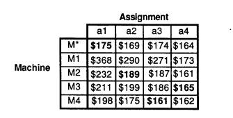
Table
A3 gives the results of all the calculations done to complete the matrix showing
the effective cost of working all available loaders in all possible assignments.
|
TABLE A3.-Results from reassignment model |
|
|
Although
they are not shown here, there are a number of standard operations research
techniques available to choose assignments in a manner which minimizes the total
cost in the matrix above. The minimum cost assignments are shown in bold type in
Table A3.
From
this it can be seen that:
|
Appendix II. �
References
|
Appendix
III: Notation
The
following symbols are used in this paper:
|
Subscripts
|