-
ASC Proceedings of the 42nd Annual Conference
-
Colorado State University Fort Collins, Colorado
-
April 20 - 22, 2006
|
|
|
Stochastic Prediction of Design Costs for Transportation Projects
|
Mohamed Y. Hegab, Ph.D., P.E. California State University-Northridge Northridge, California |
Khaled M. Nassar, Ph.D. University of Maryland Eastern Shore Princess Ann, Maryland |
|
Transportation projects are usually designed in three phases. Phase I is the preliminary design report and all its necessary documents, Phase II involves the preparation of the actual construction documents, including plans and specifications, and Phase III involves the construction inspection and project’s contract administration. The process of arriving at total person-hours and design costs for Phase II to perform the work is often tedious for both the consultant and the department of transportation (DOT). A major drawback of this process is that the design cost is often reached using heuristic evaluation and without any scientific basis. From the DOT District’s viewpoint, consultant’s hours often seem inflated with the hopes of getting more hours than required to perform the job, while the consultant thinks the District is being unrealistic. The main objective of this research is to model the design costs on consultant-designed projects. Actual data were collected from The Illinois Department of Transportation (IDOT). Stochastic modeling techniques were then used to predict the design costs. The models developed will help supplement the current methods of estimating design costs used by IDOT and help provide better estimates. The models contained in this research can be implemented in the Design and Environment manuals of IDOT. They can also be used as guide for other states’ DOTs.
Key Words: Design Cost, Transportation Projects, Construction, Stochastic Analysis, Probability Distribution. |
Introduction
Activities of the Design Process
The general procedure for hiring a consulting firm for a Phase II job involves several steps. Step 1 is when Illinois Department of Transportation (IDOT) advertises the project in the Professional Transportation Bulletin (IDOT, 2002). The Professional Transportation Bulletin is a publication published by IDOT listing all of the upcoming projects for which consultants can submit statements of interest. In Step 2, several consulting “firms” will submit statements of interest to IDOT for a particular job. These documents will outline the firms desire to perform the work and summarize their qualifications to do the work. Step 3 is when IDOT confirms the eligibility of each consultant who submits a statement of interest. In Step 4, IDOT will perform a preliminary review and rank each firm. A consultant-selection committee will then determine which firm is awarded the job. After a firm is selected, IDOT notifies the selected firm.
After a firm is selected for a particular job, several more steps must be completed prior to beginning actual design work. An initial meeting is held with the District to discuss the scope of the project. The consultant then returns to his office to enumerate tasks and estimate the number of person-hours needed to complete the job. Design firms usually rely only on activity-analysis methods of engineering estimates, (Hudgens & Lavelle 1995). This is a very common method also used by engineering firms performing work for IDOT. As an example of activity-analysis, a consulting firm calculates the amount of time required to produce a typical section. The consultant will then submit these person-hours to the District. The last step is getting the person-hours finalized so that both parties agree on the total projected hours and design costs.
There are two main problems. First, the process of arriving at total person-hours and design costs to perform the work is often painful for both the consultant and IDOT. From the District’s viewpoint, consultant’s hours often seem to be inflated with the hopes of getting more hours than required to perform the job, while the consultant thinks the District is being unrealistic. Second, the submittal from the consultant to the District will include the number of person-hours per task as broken down by the consultant. Each individual consultant may break the hours down differently. As a result, it is difficult to compare person-hours per task per consultant per job. Another factor, which enters the Phase II design process, is called “the complexity factor.” Every Professional Transportation Bulletin advertisement has a complexity factor assigned to each job. This factor, as its name suggests, is a numerical value based on its anticipated difficulty to design, as shown in Table 1 (IDOT, 2002).
Table 1
Complexity Factors
|
LOW COMPLEXITY .000 (1) |
MEDIUM COMPLEXITY .035 (2) |
HIGH COMPLEXITY .070 (3) |
|
Location/Design Report |
Location/Design Report (Reconstruction/Major Rehabilitation) |
Location/Design Report (New Construction/Major Reconstruction) |
|
SEA |
CEA |
EIS |
|
Small Rural Projects |
Small Urban Projects |
Major Urban Freeways |
|
Surveys |
Freeways |
Multi-level Interchanges |
|
Roads and Streets |
Freeway interchanges |
Highway Structures: Advanced Typical |
|
Highway Structures: Simple |
Projects on New Alignment |
Highway Structures: Complex |
|
Construction Engineering (Rural Freeway) |
Construction Engineering(Urban Freeway & Major Structures) |
Major River Bridges |
|
Traffic Signals |
Highway Structures: Typical |
Movable Bridges |
|
Lighting |
Railroad Structures |
Major Engineering Studies Requiring Special Expertise |
|
Aerial Mapping |
Traffic Signals (SCAT) |
Traffic Signals with Railroad Interconnect |
|
Asbestos Abatement |
Hazardous Waste |
Hydraulic Reports, Waterway: Complex |
|
Pumping Stations |
Hydraulic Reports, Waterways: Typical |
Quality Assurance: Complex |
|
Subsurface Utility Engineering |
Hydraulic Reports, Pump Stations |
Bituminous Mix Designs: Complex |
|
|
Quality Assurance: Typical |
Geotechnical Engineering: Complex |
|
|
Bituminous Mix Designs: Typical |
|
|
|
Geotechnical Engineering: Typical |
|
Data Collection and Analysis
Data extracted from IDOT databases cover fifty-nine projects from different Districts of IDOT. They include design costs (DC), programmed costs (initial planned construction costs) (PC), complexity factors (CF), percentage of bridges in projects (BR), and percentage of roadways in projects (RD). BR and RD were calculated as a percentage of cost.
The data collected were for projects covering a wide range of costs up to $18 Million. In order to develop a mode accurate model, the design cost data were clustered into three different data bands; low design cost, average design costs and high design costs. After clustering the data, the different data clusters were divided into two sets. One of those sets will be used to develop the model and the other will be used for testing. The two data sets were selected by assigning random numbers and then sorting in an ascending order. The first 15% of the data were selected for model testing and the remaining 85% for model development. The same procedure was applied to each of three data clusters.
In order to develop the design cost model stochastic analysis was performed. Stochastic analysis is a statistical technique that takes into consideration the probabilities of estimated cost. This analysis is usually performed on a number of stages: choosing the appropriate probabilistic distribution of design costs, building a prediction model for design costs, and model validation.
.
Choosing Probability Distribution
A probability distribution of a variable is a representation of probabilities associated with each of the possible values of the variable. A number of probability distributions were used to represent design costs. Those considered were Weibull, Lognormal base e, Exponential, Normal, Extreme Value, Lognormal base 10, Logistic, and Loglogistic distributions. These distributions have one or two parameters to represent its shape and scale, (Hosmer and Lemeshow 1999).
To select the appropriate probabilistic shape for design costs data, a probability plot of the data were drawn. A distribution probability plot is a plot of the studied variable to test if a given set of the variable’s data follows the specified distribution. The probability plot should be approximately linear if the specified distribution is the correct model. Various distributions were compared to the design costs data. When the design costs’ plotted points hold close to the fitted line, the candidate distribution fits the data adequately. Anderson-Darling (AD) goodness-of-fit measure was used to compare the fit of different distributions to the data. Lower AD values indicate a better fitting distribution than higher AD values, (Hosmer and Lemeshow 1999). The data plots for different probability distributions are shown in Figure 1 and Table 2 shows AD values for these distributions. Because the Lognormal base e distribution has the lowest AD value, it was selected.
Building a prediction model
From the above analysis, the data seem to fit a lognormal distribution. Since traditional regression analysis assumes a normal distribution of the data, another type of regression called “Regression with Life Data” was used to develop the design cost model. “Regression with Life Data” is used with data that follow any known distribution other than normal, (Meeker and Escobar, 1998) and transforms the lognormal base e distribution to the following linear form:
Table 2
Comparing AD values of different probability distributions
|
Distribution (1) |
AD value (2) |
Remarks (3) |
|
1.221 |
|
|
|
Lognormal base e |
0.836 |
Best fitting candidate |
|
Exponential |
1.191 |
|
|
Normal |
4.218 |
|
|
Lognormal base 10 |
0.836 |
|
|
Extreme Value |
6.207 |
|
|
Loglogistic |
0.93 |
|
|
Logistic |
3.336 |
|
|
|
|
|
“Regression with Life Data” was performed using MINITAB 13.3 software assuming lognormal base e distribution of design costs. The results of the analysis, as shown in Table 3, show that the p-value is lower than the a-value (0.05). As a result, initial planned construction costs (PC), complexity factors (CF), and percentage of roadways in projects (RD) are significant variables in predicting design cost with a 95% confidence limit. The design cost is:
 |
|
where, |
DC = Design costs ($)
PC = programmed costs (initial planned construction costs) ($)
CF = complexity factors
BR = percentage of bridges in projects (%)
RD = percentage of roadways in projects (%)
Based in the above analysis, three models can be developed from the first quartile, median, and third quartile of the probability distribution. All data were used to predict the general form of models, which depends on the required percentile of occurrence. The developed models were based on probability of 25, 50, and 75 percentile. The models, which are labeled low cost, average cost, and high cost design, are as follows:
|
|
|
|
|
|
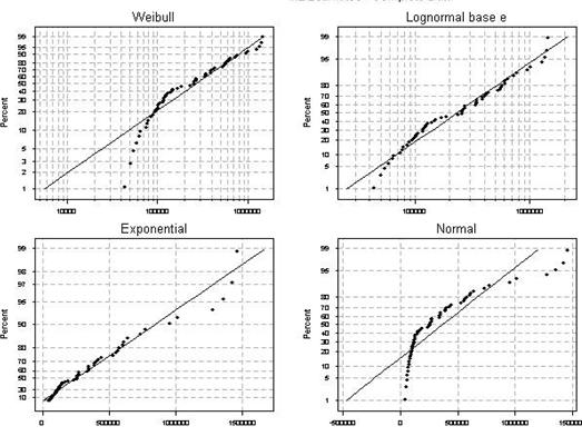 |
| Figure 1: Comparison between different probability plots to fit design cost data (horizontal axis is design cost and vertical axis is cumulative probability) |
The models do not have upper boundaries for the size of projects but it is preferable to be within limits of data ($18 Millions). The models are graphically represented in Figure 2 for a hypothetical project.
 |
| Figure 2: Design cost models for difference levels |
Model Validation using residuals
To test the validity of the model, residuals should be checked. According to Meeker and Escobar (1998), residuals should follow the Normal distribution when the model parameter follows a lognormal base e distribution. Residuals are represented by the error term ep. The probability plot for the model residuals based on Normal distribution is shown in Figure 3. The AD measure of the residuals’ compatibility to the Normal distribution was 1.0277 (the lower, the better). The AD value, which is used for comparison between different models, has an acceptable value of ±3. One can likely assume residuals can follow the Normal distribution while design costs can follow the Lognormal base e distribution.
Table 3
Results of “Regression with Life Data” for design cost
|
Estimation Method: Maximum Likelihood Distribution: Lognormal Base e
95.0% Normal CI Intercept 11.5976 0.1356 85.50 0.000 11.3317 11.8634 PTB 1.0939E-07 1.9245E-08 5.68 0.000 7.1665E-08 1.4710E-07 CF 10.737 5.117 2.10 0.036 0.707 20.767 Rd 0.4720 0.2212 2.13 0.033 0.0384 0.9056 Scale 0.62221 0.05777 0.51868 0.74639 Log-Likelihood = -771.464 Anderson-Darling (adjusted) Goodness-of-Fit Standardized Residuals = 0.83 |
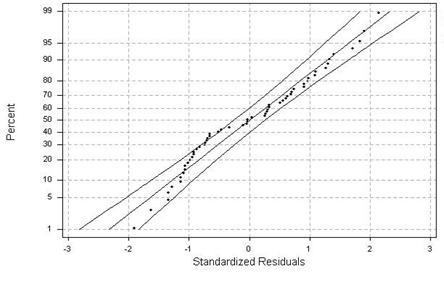 |
| Figure 3: Probability plot of residuals –Normal distribution with 95% CI (Confidence Interval) (horizontal axis is standardized residual and vertical axis is cumulative probability) |
Summary
In this paper, a model for design costs of transportation projects was developed as a function of initial construction cost, complexity factor, and percentage of highways in the project. A representative probability distribution was selected for the design costs. After investigating different probability distributions, lognormal base e distribution was selected. “Regression with Life Data” was used to predict design costs. After modeling the design cost, residuals were used to check if the selected distribution fits the model. The model seems to perform well on the test data and has several uses.
Design cost models can be used as control charts for engineers’ costs. IDOT can calculate the design cost limits of a project, fit different quotes from engineers in the graph (Figure 3), and evaluate proposals. Other DOTs can use this model for guidance, but an individual model for each DOT should be developed.
Reference
Hosmer D., & Lemeshow, S. (1999). Applied Survival Analysis: Regression Modeling of Time to Event Data, New York: Wiley Series in Probability and Statistics.
Hudgins, D. W., and Lavelle, J. P. (1995). Estimating Engineering Design Costs, Engineering Management Journal, 7 (3), 17-23.
IDOT (2002). Consultants Professional Transportation Bulletin, Illinois: Illinois Department of Transportation.
Meeker, W., & Escobar, L. (1998). Statistical Methods for Reliability, (2nd ed.), New York: Wiley Series in Probability and Statistics.
